THE ABILITY OF WINNERS TO WIN AGAIN

Even people who aren’t avid baseball fans (your DSN editor included) can get something out of this one.
When two baseball teams play each other on two consecutive days, what is the probability that the winner of the first game will be the winner of the second game?
[If you like fun, write down your prediction.]
DSN’s father-in-law told him that recently the Mets beat the Phillies 9 to 1, but the very next day, the Phillies beat the Mets 10 to 0. How could this be? If the Mets were so good as to win by 8 points, how could the exact same players be so bad as to lose by 10 points to the same opponents 24 hours later?
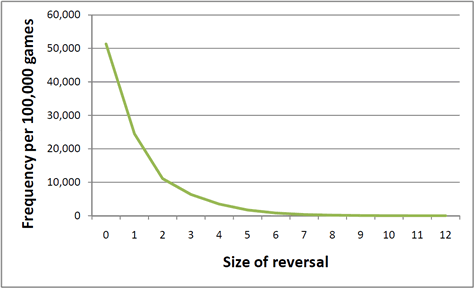
Let’s call this situation (in which team A beats team B one one day, but team B beats team A the very next day) a “reversal”, and we’ll say the size of the reversal is the smaller of the two margins of victory. In the above example, the size of the reversal was 8.
Using R (code provided below), DSN obtained statistics on all major league baseball games played between 1970 and 2009 and calculated how often each type of reversal occurs per 100,000 pairs of consecutive games. The result is in the the graph above. Big reversals are rare. A reversal of size 8 occurs in only 174 of 100,000 games; a size 12 reversal happens but 10 times per 100k. A size 13 reversal never happened in those 40 years. One might think this is because it would be uncommon for a team that is so good to suddenly become so bad and vice versa, but note that big margins of victory are rare: only 4% of games have margins of victory of 8 points or larger.
Back to our question:
If a team wins on one day, what’s the probability they’ll win against the same opponent when they play the very next day?
We asked two colleagues knowledgeable in baseball and the mathematics of forecasting. The answers came in between 65% and 70%.
The true answer: 51.3%, a little better than a coin toss.
That’s right. When you win in baseball, there’s only a 51% chance you’ll win again in more or less identical circumstances. The careful reader might notice that the answer is visible in the already mentioned chart. The reversals of size 0, (meaning no reversal, meaning the same team won twice) occur 51,296 times per 100,000 pairs of consecutive games.
[At this point, DSN must admit that it is entirely possible that it has made a computational error. It welcomes others to reproduce the analysis with the code or pre-processed data at the end of this post.]
What of the adage “the best predictor of future performance is past performance”? It seems less true than Sting’s observation “History will teach us nothing“. Let’s continue the investigation.
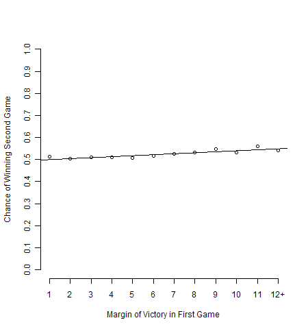
Here were plot the probability of winning the second game based on obtaining various margins of victory in the first game. We simply calculated the average win rate for each margin of victory up to 11 games, which makes up 98% of the data, and bin together the remaining 2%, comprising margins of victory from 12 to 27 points. (Rest assured, the binning makes the graph look prettier, but does not affect the outcome.)

The equation of the robust regression line is: Probability(Win_Second_Game) = .498 + .004*First_Game_Margin which suggests that even if you win the first game by an obscene 20 points, your chance of winning the second game is only 57.8%
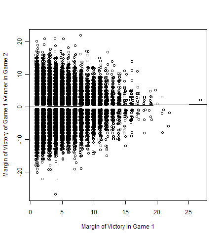
Still in disbelief? Here we do no binning and plot the margin of victory (or loss) of the first game winner as a function of its margin of victory in the first game. The clear heteroskedasticity is dealt with by iterative reweighted least squares in R’s rlm command. Similar results are obtained by fitting a loess line. This model is Expected_Second_Game_Margin = -.012 + .030*First_Game_Margin

One final note. The 51.3% chance you’ll win the second game given you’ve won the first is smaller than the so called “home team advantage”, which we found to be a win probability of 54.2% on first games and 53.8% on second games.
When the home team wins the first game, it wins the second game 54.7% of the time.
When the home team loses the first game, it wins the second game 52.8% of the time.
When the visitor wins the first game, it wins the second game 47.2% of the time.
When the visitor loses the first game, it wins the second game 45.3% of the time.
Surprisingly, when it comes to winning the second game, it’s better to be the home team who just lost than the visitor who just won. So much for drawing conclusions from winning. Decision Science News has always wondered why teams are so eager to fire their coaches after they lose a few big games. Don’t they realize that their desired state of having won those same few big games would have been mostly due to luck?
There you have it. Either we have made an egregious error in calculation or recent victories are surprisingly uninformative.
Do your own analysis alternative 1: The pre-processed data
If you wish, you can cheat and get the pre-processed data at http://www.dangoldstein.com/flash/bball/reversals.zip
This may be of interest for people who don’t use R or for impatient types who just want to cut to the chase.
No guarantee that our pre-processing is correct. It should be all pairs of consecutive games between the same two teams.
Do your own analysis alternative 2: The code
I’ll provide the column names file for your convenience at http://www.dangoldstein.com/flash/bball/cnames.txt. I left out a bunch of columns names I didn’t care about. The complete list is at: http://www.dangoldstein.com/flash/bball/glfields.txt
R CODE
(Don’t know R yet? Learn by watching: R Video Tutorial 1, R Video Tutorial 2)
#Data obtained from http://www.retrosheet.org/
#Go for the files http://www.retrosheet.org/gamelogs/gl1970_79.zip through
#http://www.retrosheet.org/gamelogs/gl2000_09.zip and unzip each to directories
#named "gl1970_79", "gl1980_89", etc, reachable from your working directory.
library(MASS) #For robust regression, can omit if you don't want to fit lines
#Column headers, Can get from www.dangoldstein.com/flash/bball/cnames.txt
#If you want all the headers, create from www.dangoldstein.com/flash/bball/glfields.txt
LabelsForScript=read.csv("cnames.txt", header=TRUE)
#Loop to get together all data
dat=NULL
for (baseyear in seq(1970,2000,by=10))
{
endyear=baseyear+9
#string manupulate pathnames
#reading in datafiles to one big dat goes here
for (i in baseyear:endyear)
{
mypath=paste("gl",baseyear,"_",substr(as.character(endyear),start=3,stop=4),"/GL",i,".TXT",sep="")
cat(mypath,"\n")
dat=rbind(dat,read.csv(mypath, col.names=LabelsForScript$Name))
}
}
rel=dat[,c("Date", "Home","Visitor","HomeGameNum","VisitorGameNum","HomeScore","VisitorScore")] #relevant set
rel$PrevVisitorGameNum=rel$VisitorGameNum-1
rel$PrevHomeGameNum=rel$HomeGameNum-1
rel$year=substr(rel$Date,start=1,stop=4)
rm(dat)
head(rel,20); summary(rel)
relmerge=merge(rel,rel,
by.x=c("Home","Visitor","year","HomeGameNum","VisitorGameNum"),
by.y=c("Home","Visitor","year","PrevHomeGameNum","PrevVisitorGameNum")
)
relmerge=relmerge[,c(
"Home", "Visitor", "Date.x", "HomeScore.x", "VisitorScore.x",
"Date.y", "HomeScore.y", "VisitorScore.y"
)]
relmerge$dx=relmerge$HomeScore.x-relmerge$VisitorScore.x
relmerge$dy=relmerge$HomeScore.y-relmerge$VisitorScore.y
#Eliminate ties
relmerge=with(relmerge,relmerge[(dx!=0) & (dy!=0),])
relmerge$reversal=-.5*(sign(relmerge$dx)*sign(relmerge$dy))+.5
relmerge$revsize=relmerge$reversal*pmin(abs(relmerge$dx),abs(relmerge$dy))
relmerge$winnerMarginVicG1=with(relmerge,sign(dx)*dx)
relmerge$winnerMarginVicG2=with(relmerge,sign(dx)*dy)
write.csv(relmerge,"reversals.csv")
mat=NULL
mat= data.frame(cbind(
ReversalSize=0:12,
Count=table(relmerge$revsize),
Prob=table(relmerge$revsize)/length(relmerge$revsize),
Per100k=table(relmerge$revsize)/length(relmerge$revsize)*100000
))
mat
cat("Probability previous winner wins again: ", mat[1,3],"\n")
##Graph Size of Reversal Frequency
png("SizeOfReversal.png",width=450)
plot(mat$ReversalSize,mat$Per100k,xlab="Size of Reversal",ylab="Frequency in 100,000 games",type="lines")
dev.off()
##Graph Chance of Winning Given Previous Win of Various Margins
png("WinGivenMargin.png",width=450)
brks=cut(relmerge$winnerMarginVicG1,breaks=c(0,1,2,3,4,5,6,7,8,9,10,11,27))
winsVsMargin=tapply(relmerge$winnerMarginVicG2>0,brks,mean)
names(winsVsMargin)=1:12
plot(winsVsMargin,ylim=c(0,1),axes=FALSE,xlab="Margin of Victory in First Game",ylab="Chance of Winning Second Game")
axis(1,1:12,labels=c("1","2","3","4","5","6","7","8","9","10","11","12+"))
axis(2,seq(0,1,.1))
winModel=rlm(winsVsMargin~ as.numeric(names(winsVsMargin)))
abline(winModel)
dev.off()
##Graph Expected Margin of Victory Given Past Margin of Victory
png("MarVic.png",width=450)
mm2=rlm(relmerge$winnerMarginVicG2 ~ relmerge$winnerMarginVicG1)
plot(jitter(relmerge$winnerMarginVicG1),
jitter(relmerge$winnerMarginVicG2),xlab="Margin of Victory in Game 1",
ylab="Margin of Victory of Game 1 Winner in Game 2")
abline(mm2)
dev.off()
#Probability of team winning game two if they won game 1 by n points
winModel$coefficients[1]+winModel$coefficients[2]*20
#Expected margin of victory in game two given win in game 1
mm2$coefficients[1]+mm2$coefficients[2]*33
#Home Team Advantage: First game, second game
with(relmerge,{cat(mean(dx > 0), mean(dy > 0))})
#Home team advantage second game given home won first game
# Equals 1- Visitor p win second game given visitor lost the first game
with(relmerge[relmerge$dx > 0,],mean(dy > 0))
#Home team advantage second game given home lost first game
#Equals 1 - Visitor p win second game given visitor won first game
with(relmerge[relmerge$dx < 0,],mean(dy > 0))
This entry was posted on Wednesday, May 5th, 2010.
 Subscribe to Decision Science News by Email (one email per week, easy unsubscribe)

