Dollars and cents: How are you at estimating the total bill?
ROUNDING HEURISTICS AND THE DISTRIBUTION OF CENTS FROM 32 MILLION PURCHASES
When estimating the cost of a bunch of purchases, a useful heuristic is rounding each item to the nearest dollar. (In fact, on US income tax returns, one is allowed to round and not report the cents). If prices were uniformly distributed, the following two heuristics would be equally accurate:
* Rounding each item up or down to the nearest dollar and summing
* Rounding each item down, summing, and adding a dollar for every two line items (or 50 cents per item).
But are prices uniformly distributed? Decision Science News wanted to find out.
Fortunately, our Alma Mater makes publicly available the famous University of Chicago Dominick’s Finer Food Database, which will allow us to answer this question (for a variety of grocery store items at least).
We looked at over 32 million purchases comprising:
* 4.8 million cereal purchases
* 2.2 million cracker purchases
* 1.7 million frozen dinner purchases
* 7.2 million frozen entree purchases (though we’re not sure how they differ from “dinners”)
* 4.1 million grooming product purchases
* 4.3 million juice purchases
* 3.3 million laundry product purchases and
* 4.7 million shampoo purchases
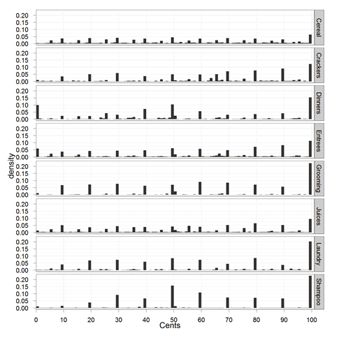
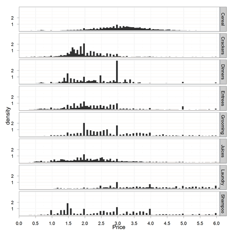
The distribution of their prices can be seen above. But what about the cents? We focus down on them here:

As is plain, there are many “9s prices” — a topic well-studied by our marketing colleagues — and there are more prices above 50 cents then below it. The average number of cents turns out to be 57 (median 59).
In sum (heh), it pays to round properly, though we do think some clever heuristics can exploit the fact that each dollar has on average 57 cents associated with it.
Anyone who wants our trimmed down, 11 meg, version of the Dominick’s database (just these categories and prices) is welcome to it. It can be downloaded here: http://dangoldstein.com/flash/prices/.
Plots are made in the R language for statistical computing with Hadley Wickham’s ggplot2 package. The code is here:
if (!require("ggplot2")) install.packages("ggplot2")
library(ggplot2)
orig = read.csv("prices.tsv.gz", sep = "\t")
summary(orig)
orig$cents = orig$Price - floor(orig$Price)
#sampledown
LEN = 1e+06
prices = orig[sample(1:nrow(orig), LEN), ]
prices$cents = round((prices$Price - floor(prices$Price)) *
    100, 0)
summary(prices)
p = ggplot(prices, aes(x = Price)) + theme_bw()
p + stat_bin(aes(y = ..density..), binwidth = 0.05,
    geom = "bar", position = "identity") + coord_cartesian(xlim = c(0,
    6.1)) + scale_x_continuous(breaks = seq(0, 6, 0.5)) +
    scale_y_continuous(breaks = seq(1,
    2, 1)) + facet_grid(Item ~ .)
ggsave("prices.png")
p = ggplot(prices, aes(x = cents)) + theme_bw()
p + stat_bin(aes(y = ..density..), binwidth = 1, geom = "bar",
    position = "identity",right=FALSE) + coord_cartesian(xlim = c(0, 100)) +
    scale_x_continuous(name = "Cents", breaks = seq(0, 100, 10)) +
    facet_grid(Item ~ .)
ggsave("cents.png")


[…] this link: How are you at estimating the amount bill? | Decision Science News Share and […]
October 1, 2011 @ 12:11 am
Can you say, “Benford’s Law”?
October 1, 2011 @ 10:06 am
Bruce: Benford’s predicts that 9 would be the least common number. In these data, it’s the most common number.
October 1, 2011 @ 2:53 pm
For the first line of code, I usually use
if (!require('ggplot2')) install.packages('ggplot2')Then you may use formatR to tidy up the code (https://github.com/yihui/formatR/wiki), and put them in the pre tag instead of code tag.
Thanks for introducing this great dataset!
October 1, 2011 @ 2:25 pm
Brilliant as always, Yihui.
October 1, 2011 @ 2:54 pm
[…] commenter on our last post brought up Benford’s law, the idea that naturally occurring numbers follow a predictable […]
October 5, 2011 @ 3:26 pm