Do cents follow Benford’s Law?
MANY THINGS FOLLOW BENFORD’S LAW. CENTS DON’T.
A commenter on our last post brought up Benford’s law, the idea that naturally occurring numbers follow a predictable pattern. Does Benford’s law apply to the cent amounts taken from our 32 million grocery store prices?
Benford’s law, if you don’t know about it, is an amazing thing. If you know the probability distribution that “natural” numbers should have, you can detect where people might be faking data: phony tax returns, bogus scientific studies, etc.
In Benford’s law, the probability of the leftmost digit of a number being d is
log10(d + 1) – log10(d)
(according to the Wikipedia page, anyway).
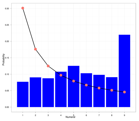
In the chart above, we plot the predictions of Benford’s law in red points. The distribution of leftmost digits in our cents data is shown in the blue bars.
As the chart makes plain, cents after the dollar do not seem distributed in a Benford-like manner. And no one is “faking” cents data. It is simply that Benford’s is a domain specific heuristic. Grocery store prices seem to be chosen strategically. Look at all those nines. Perhaps dollar (as opposed to cent) prices in the grocery store are distributed according to Benford, but we leave that as an exercise for the reader.
Want to play with it yourself? The R / ggplot2 code that made this plot is below, and the anyone who wants our trimmed down, 12 meg, version of the Dominick’s database (just these categories and prices) is welcome to it. It can be downloaded here: http://dangoldstein.com/flash/prices/.
if (!require("ggplot2")) install.packages("ggplot2")

orig = read.csv("prices.tsv.gz", sep = "\t")
orig$cents = round(100 * orig$Price)%%100
# First digit
orig$fd = with(orig, ifelse(cents < 10, round(cents), cents%/%10))
sumif = function(x) {sum(orig$fd == x)}
vsumif = Vectorize(sumif)
df = data.frame(Numeral = c(1:9), count = vsumif(1:9))
df$Probability = df$count/sum(df$count)
ben = function(d) {log10(d + 1) - log10(d)}
df$benford = ben(1:9)
p = ggplot(df, aes(x = Numeral, y = Probability)) + theme_bw()
p = p + geom_bar(stat = "identity", fill = I("blue"))
p = p + scale_x_continuous(breaks = seq(1:9))
p = p + geom_line(aes(x = Numeral, y = benford, size = 0.1))
p = p + geom_point(aes(x = Numeral, y = benford, color = "red", size = 1))
p + opts(legend.position = "none")
ggsave("benford.png")
ADDENDUM 1:
Plyr / ggplot author Hadley Wickham submitted some much prettier Hadleyfied code, which I studied. It wasn't quite counting the same thing my code counts, so I modified it so that they do the same thing. Most of the difference had to do with rounding. The result is here:
orig2 <- read.csv("prices.tsv.gz", sep = "\t")
orig2 <- mutate(orig2,
  cents = round(100 * Price) %% 100,
  fd = ifelse(cents<10,round(cents),cents %/% 10))
df2 <- count(orig2, "fd")
df2 <- mutate(df2,
  prob = prop.table(freq),
  benford = log10(fd + 1) - log10(fd + 0))
ggplot(df2, aes(x = fd, y = prob)) +
  geom_bar(stat = "identity", fill = "blue") +
  geom_line(aes(x = fd, y = benford, size = 0.1)) +
  geom_point(aes(x = fd, y = benford, color = "red", size = 1)) +
  theme_bw()
  scale_x_continuous(breaks = seq(1:9))
Playing with system.time() if found that the "mutate" command in plyr is slightly faster than my two calls to modify "orig" and much more compact. Lesson learned: Use mutate over separate calls and over "tranform".
My application of calls to sum(orig$fd==x) is faster than Hadley's count(orig2, "fd"), however "count" is much more general purpose and faster than "table" according to my tests, so I will be using it in the future.
ADDENDUM 2:
Big Data colleague Jake Hofman proves that awk can do this much faster than the R code above:
zcat prices.tsv.gz | awk 'NR > 1 {cents=int(100*$2+0.5) % 100;
counts[substr(cents,1,1)]++} END {for (k in counts) print k,
counts[k];}' > benford.dat
Jake's code runs in about 20 seconds, mine and Hadley's runs in about a minute.


Nice charts and code, but — isn’t this a priori a situation where Benford’s Law is unlikely? I don’t think it has too much to do with the 9’s… Rather, as Wikipedia states, “It tends to be most accurate when values are distributed across multiple orders of magnitude.” Since cents are guaranteed to be in the range 1-99, i.e. across only two orders of magnitude, I’d be surprised if you *did* see a Benford-like distribution.
October 5, 2011 @ 5:29 pm
Jerzy, agreed! But I did want to follow up on that comment from the last post.
October 5, 2011 @ 5:45 pm
[…] example here: Do cents study Benford's Law? | Decision Science News Share and […]
October 5, 2011 @ 6:54 pm
I’ve found that house numbers follow Benford’s Law. It was an example given from the Wikipedia page. I am currently looking at member subscription data and found that categories of certain members that deviated from Benford’s Law distribution were more fraudulent. It is a very interesting phenomenon.
October 6, 2011 @ 10:05 am
The key to Benford’s Law is that it is a law for first digits. There are generalised (and less-impressive) laws for second digits, etc. I’d see cents as effectively the second last digit, by which stage the distribution should be pretty close to uniform. So what you’re seeing here is essentially a uniform distribution overlaid with a .99 effect boosting 9s.
April 16, 2012 @ 7:11 pm