You’ve got the whole world in your portfolio
LEARN HOW TO IMPORT WORLD BANK DATA AND INVEST IN THE WHOLE WORLD

Click to enlarge
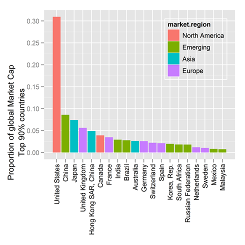
The market cap of the countries comprising 90% of the world’s market cap (end 2010)
A famous finance professor once told us that good diversification meant holding everything in the world. Fine, but in what proportion?
Suppose you could invest in every country in the world. How much would you invest in each? In a market-capitalization weighted index, you’d invest in each country in proportion to the market value of its investments (its “market capitalization”). As seen above, the market-capitalization of the USA is about 30%, which would suggest investing 30% of one’s portfolio in the USA. Similarly, one would put 8% in China, and so on. All this data was pulled from the World Bank, and at the end of this post we’ll show you how we did it.
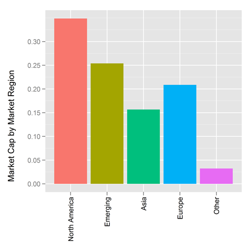
What makes life easy is that economists have grouped countries into regions and the market caps of each can be computed by summing the market caps of the constituent countries. See this MSCI page for the manner in which we’ve categorized countries in this post:
North America: USA, Canada
Emerging: Brazil, Chile, China, Colombia, Czech Republic, Egypt, Hungary, India, Indonesia, Korea, Malaysia, Mexico, Morocco, Peru, Philippines, Poland, Russia, South Africa, Taiwan, Thailand, Turkey
Asia: Japan, Australia, Hong Kong, New Zealand, Singapore
Europe: Austria, Belgium, Denmark, Finland, France, Germany, Greece, Ireland, Italy, Netherlands, Norway, Portugal, Spain, Sweden, Switzerland, United Kingdom
Other: Everybody else in the world
What makes life easier still is that one can purchase ETFs that work like indices tracking the various regions of the world. For example at Vangard one can purchase
- Vanguard Total Stock Market ETF (Ticker VTI), which basically covers North America
- Vanguard MSCI Emerging Marketing ETF (Ticker VWO), which covers emerging markets
- Vanguard MSCI Pacific ETF (Ticker VPL), which covers Asia (minus the Asian emerging markets countries)
- Vanguard MSCI Europe ETF (Ticker VGK), which covers Europe
What makes life a bit more complicated is that not everybody agrees on market-cap weighting. Some favor Gross Domestic Product (GDP) weighting for the reasons given at this MSCI page.
- GDP figures tend to be more stable over time compared to equity markets’ performance-related peaks and troughs
- GDP weighted asset allocation tends to have higher exposure to countries with above average economic growth, such as emerging markets
- GDP weighted indices may underweight countries with relatively high valuation, compared to market-cap weight indices
Here are the countries that make up 90% of the world’s GDP:

Click to enlarge
The GDP of the countries comprising 90% of the world’s GDP (end 2010)
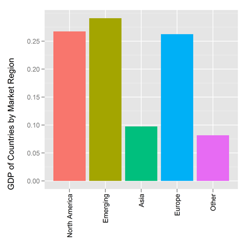
Because we love you, we’ve also computed how the classic market regions compare to one another in terms of GDP
If you track changes in market cap from month to month as we do, you’ll appreciate the stability that GDP weighting provides. For example, the market cap data in this post, from 2010, is already way out of date.
So, weight by market cap, or weight by GDP, or do what we do and weight by the average of market cap and GDP, but don’t wait to diversify your portfolio outside of a handful of investments you happen to own. Invest in the world.
For those who love R and who want to learn how to pull down World Bank data, the code is provided here. I got started with this by borrowing code from this very helpful blog post by Markus Gesmann and tip my hat to its author. Thanks also to Hadley for writing ggplot2 (and for visiting us at Yahoo the other week. And thanks to Yihui Xie for his code formatter.
R CODE
library(ggplot2)

library(car)

library(RJSONIO)

ftse=read.delim("201112_FTSE_Market_Caps.tsv",sep="\t")

##See www.msci.com/products/indices/tools/index.html

##Emerging::Brazil, Chile, China, Colombia, Czech Republic, Egypt, Hungary,

#India, Indonesia, Korea, Malaysia, Mexico, Morocco, Peru, Philippines,

#Poland, Russia, South Africa, Taiwan, Thailand, Turkey

##Europe::Austria, Belgium, Denmark, Finland, France, Germany, Greece, Ireland, Italy,

#Netherlands, Norway, Portugal, Spain, Sweden, Switzerland, United Kingdom

##Asia::Japan, Australia, Hong Kong, New Zealand, Singapore

recodestring="   c('USA','CAN')='North America';

                 c('BRA','CHL','CHN','COL','CZE','EGY','HUN','IND','IDN','KOR','MYS','MEX','MAR','PER','PHL','POL',

                  'RUS','ZAF','TWN','THA','TUR')= 'Emerging';

                 c('AUT','BEL','DNK','FIN','FRA','DEU','GRC','IRL','ITA',

                  'NLD','NOR','PRT','ESP','SWE','CHE','GBR')= 'Europe';

                  c('JPN','AUS','HKG','NZL','SGP')= 'Asia';

                  else='Other'"

#How much of the world do we want to consider (to keep graphs manageable)

CUTOFF=.9

#Some code from internet to read world bank data. Adapted from

#http://www.r-bloggers.com/accessing-and-plotting-world-bank-data-with-r/

#See also http://data.worldbank.org/indicator/NY.GDP.MKTP.CD

getWorldBankData = function(id='NY.GDP.MKTP.CD', date='2010:2011',

                            value="value", per.page=12000){

  require(RJSONIO)

  url = paste("http://api.worldbank.org/countries/all/indicators/", id,

              "?date=", date, "&format=json&per_page=", per.page,

              sep="")

  wbData = fromJSON(url)[[2]]

  wbData = data.frame(

    year = as.numeric(sapply(wbData, "[[", "date")),

    value = as.numeric(sapply(wbData, function(x)

      ifelse(is.null(x[["value"]]),NA, x[["value"]]))),

    country.name = sapply(wbData, function(x) x[["country"]]['value']),

    country.id = sapply(wbData, function(x) x[["country"]]['id'])

    )

  names(wbData)[2] = value

  return(wbData)

}

getWorldBankCountries = function(){

  require(RJSONIO)

  wbCountries =

    fromJSON("http://api.worldbank.org/countries?per_page=12000&format=json")

  wbCountries = data.frame(t(sapply(wbCountries[[2]], unlist)))

  levels(wbCountries$region.value) = gsub("\\(all income levels\\)",

                                          "", levels(wbCountries$region.value))

  return(wbCountries)

}

### Get the most recent year with data

curryear = as.numeric(format(Sys.Date(), "%Y"))

years = paste("2010:", curryear, sep="")

##Get GDP for the countries (GDP in Current US Dollars)

GDP = getWorldBankData(id='NY.GDP.MKTP.CD',

                                date=years,

                                value="gdp")

#If a year has > 60 NAs it is not ready

while(  sum(is.na(subset(GDP,year==curryear)$gdp)) > 60 )

  {curryear=curryear-1}

#Keep just the most current year

GDP=subset(GDP,year==curryear);

## Get country mappings

wbCountries = getWorldBankCountries()

## Add regional information

GDP = merge(GDP, wbCountries[c("iso2Code", "region.value", "id")],

                by.x="country.id", by.y="iso2Code")

## Filter out the aggregates, NAs, and irrelevant columns

GDP = subset(GDP, !region.value %in% "Aggregates" & !is.na(gdp))

GDP=GDP[,c('year','gdp','country.name','region.value','id')]

GDP=GDP[order(-1*GDP[,2]),]

GDP$prop=with(GDP,gdp/sum(gdp))

GDP$cumsum=cumsum(GDP$gdp)

GDP$cumprop=with(GDP,cumsum(gdp)/sum(gdp))

GDP$market.region=recode(GDP$id,recodestring)

resize.win <- function(Width=6, Height=6)
{
  plot.new()
  dev.off();
  #dev.new(width=6, height=6)
  windows(record=TRUE, width=Width, height=Height)
}
slice=max(which(GDP$cumprop<=CUTOFF))
smGDP=GDP[1:slice,]
smGDP$country.name=factor(smGDP$country.name,levels=unique(smGDP$country.name))
smGDP$region.value=factor(smGDP$region.value,levels=unique(smGDP$region.value))
smGDP$market.region=factor(smGDP$market.region,levels=unique(smGDP$market.region))
g=ggplot(smGDP,aes(x=as.factor(country.name),y=prop))
g=g+geom_bar(aes(fill=market.region))
g=g+opts(axis.text.x=theme_text(angle=90, hjust=1))+xlab(NULL)+
  ylab( paste("Proportion of global GDP\nTop ",CUTOFF*100,"% countries",sep=""))
g=g+opts(legend.position=c(.8,.8))
resize.win(5,5) #might have to run this twice to get it to shift from the default window
g
ggsave("GDPbyCountry.png",g,dpi=600)
smGDPsum=ddply(GDP,.(market.region),function(x) {sum(x$gdp)})
smGDPsum$V1=smGDPsum$V1/sum(smGDPsum$V1)
smGDPsum=smGDPsum[order(-1*smGDPsum[,2]),]
smGDPsum$market.region=factor(smGDPsum$market.region,levels=c("North America","Emerging","Asia","Europe","Other"))
g=ggplot(smGDPsum,aes(x=as.factor(market.region),y=V1))
g=g+geom_bar(aes(fill=market.region))
g=g+opts(axis.text.x=theme_text(angle=90, hjust=1))+xlab(NULL)+ylab("GDP of Countries by Market Region\n")
g=g+opts(legend.position="none")
resize.win(5,5) #might have to run this twice to get it to shift from the default window
g
ggsave("GDPbyRegion.png",g,dpi=600)
##Get Market Cap data from World Bank CM.MKT.LCAP.CD
### Get the most recent year with data
curryear = as.numeric(format(Sys.Date(), "%Y"))
years = paste("2010:", curryear, sep="")
##Get MarketCap for the countries (MCP in Current US Dollars)
MCP = getWorldBankData(id='CM.MKT.LCAP.CD',
                       date=years,
                       value="mcp")
#If a year has > 60 NAs it is not ready

while(  sum(is.na(subset(MCP,year==curryear)$mcp)) > 150 )

{curryear=curryear-1}

#Keep just the most current year

MCP=subset(MCP,year==curryear);

## Add regional information

MCP=merge(MCP, wbCountries[c("iso2Code", "region.value", "id")],

            by.x="country.id", by.y="iso2Code")

## Filter out the aggregates, NAs, and irrelevant columns

MCP = subset(MCP, !region.value %in% "Aggregates" & !is.na(mcp))

MCP=MCP[,c('year','mcp','country.name','region.value','id')]

MCP=MCP[order(-1*MCP[,2]),]

row.names(MCP)=NULL

MCP$prop=with(MCP,mcp/sum(mcp))

MCP$cumsum=cumsum(MCP$mcp)

MCP$cumprop=with(MCP,cumsum(mcp)/sum(mcp))

MCP$market.region=recode(MCP$id, recodestring)

slice=max(which(MCP$cumprop<=CUTOFF))
smMCP=MCP[1:slice,]
smMCP$country.name=factor(smMCP$country.name,levels=unique(smMCP$country.name))
smMCP$region.value=factor(smMCP$region.value,levels=unique(smMCP$region.value))
smMCP$market.region=factor(smMCP$market.region,levels=unique(smMCP$market.region))
g=ggplot(smMCP,aes(x=as.factor(country.name),y=prop))
g=g+geom_bar(aes(fill=market.region))
g=g+opts(axis.text.x=theme_text(angle=90, hjust=1))+xlab(NULL)+
  ylab( paste("Proportion of global Market Cap\nTop ",CUTOFF*100,"% countries",sep=""))
g=g+opts(legend.position=c(.8,.8))
resize.win(5,5) #might have to run this twice to get it to shift from the default window
g
ggsave("MCPbyCountry.png",g,dpi=600)
smMCPsum=ddply(MCP,.(market.region),function(x) {sum(x$mcp)})
smMCPsum$V1=smMCPsum$V1/sum(smMCPsum$V1)
smMCPsum=smMCPsum[order(-1*smMCPsum[,2]),]
smMCPsum$market.region=factor(smMCPsum$market.region,levels=c("North America","Emerging","Asia","Europe","Other"))
g=ggplot(smMCPsum,aes(x=as.factor(market.region),y=V1))
g=g+geom_bar(aes(fill=market.region))
g=g+opts(axis.text.x=theme_text(angle=90, hjust=1))+xlab(NULL)+ylab("Market Cap by Market Region\n")
g=g+opts(legend.position="none")
resize.win(5,5) #might have to run this twice to get it to shift from the default window
g
ggsave("MCPbyRegion.png",g,dpi=600)


The four ETFs you named from Vanguard all look reasonable, and together they cover equities from all over the world.
But as someone who works in finance, I can’t help but mention that greater diversification would include other asset classes than just equities, such as
– fixed income (bond funds)
– commodities (crude oil, gold)
– agriculture (wheat, soybeans)
However, I would NOT advise trying to get into those asset classes without careful research. Non-equity ETFs are non-trivial to construct, and sometimes they turn out not to track what they claim to track. Plus, if the ETFS are low volume, you may pay a lot in bid/ask spread.
Also, never ever touch leveraged ETFs (which claim to give you N times the return on an index such as the S&P) unless you really know what you’re doing.
December 29, 2011 @ 5:32 pm
Noted!
December 29, 2011 @ 5:34 pm
This is very neat, thanks for sharing.
What is this line supposed to be?
slice = max(which(GDP$cumprop 60 NAs it is not ready
December 30, 2011 @ 1:18 pm
Oops, I’ve fixed it
slice=max(which(GDP$cumprop<=CUTOFF))
Looks like some other stuff was messed up, too, so I repasted it all.
December 30, 2011 @ 1:29 pm
Fantastic. Thanks!
Incidentally, this was the original world bank blog post: http://lamages.blogspot.com/2011/09/accessing-and-plotting-world-bank-data.html; it’s a nice find! It is nice to link back to the original author (rather than to r-bloggers), so that they can get some traffic.
December 30, 2011 @ 1:48 pm
Fixed! Sorry, I had mistakenly linked to the r-bloggers reposting.
December 30, 2011 @ 1:57 pm
The link to Yihui’s formatR doesn’t seem to work.
great post,
Thanks
December 30, 2011 @ 8:47 pm
Ok, I’ve added a different link.
January 1, 2012 @ 1:45 pm
Hi Dan,
I am glad to see that my blog entry on “Accessing and plotting World Bank data with R” has been helpful.
Regards
Markus
January 1, 2012 @ 9:42 am
Thank you!
January 1, 2012 @ 1:43 pm
On my PC, the code does not work:
1. The variable “ftse” appears to be redundant
2. Running the code shows the following error messages
GDP$market.region=recode(GDP$id,recodestring)
Fehler in `$ resize.win slice=max(which(GDP$cumprop<=CUTOFF))
Warnmeldung:
In max(which(GDP$cumprop smGDP=GDP[1:slice,]
Fehler in 1:slice : Resultat wäre zu langer Vektor
> smGDP$country.name=factor(smGDP$country.name,levels=unique(smGDP$country.name))
Fehler in factor(smGDP$country.name, levels = unique(smGDP$country.name)) :
Objekt ‘smGDP’ nicht gefunden
> smGDP$region.value=factor(smGDP$region.value,levels=unique(smGDP$region.value))
Fehler in factor(smGDP$region.value, levels = unique(smGDP$region.value)) :
Objekt ‘smGDP’ nicht gefunden
> smGDP$market.region=factor(smGDP$market.region,levels=unique(smGDP$market.region))
Fehler in factor(smGDP$market.region, levels = unique(smGDP$market.region)) :
Objekt ‘smGDP’ nicht gefunden
> g=ggplot(smGDP,aes(x=as.factor(country.name),y=prop))
Fehler in ggplot(smGDP, aes(x = as.factor(country.name), y = prop)) :
Objekt ‘smGDP’ nicht gefunden
> g=g+geom_bar(aes(fill=market.region))
Fehler: Objekt ‘g’ nicht gefunden
> g=g+opts(axis.text.x=theme_text(angle=90, hjust=1))+xlab(NULL)+
+ ylab( paste(“Proportion of global GDP\nTop “,CUTOFF*100,”% countries”,sep=””))
Fehler: Objekt ‘g’ nicht gefunden
> g=g+opts(legend.position=c(.8,.8))
Fehler: Objekt ‘g’ nicht gefunden
> resize.win(5,5) #might have to run this twice to get it to shift from the default window
Fehler in resize.win(5, 5) : konnte Funktion “windows” nicht finden
> g
Fehler: Objekt ‘g’ nicht gefunden
> ggsave(“GDPbyCountry.png”,g,dpi=600)
Fehler in inherits(plot, “ggplot”) : Objekt ‘g’ nicht gefunden
> smGDPsum=ddply(GDP,.(market.region),function(x) {sum(x$gdp)})
Fehler: konnte Funktion “ddply” nicht finden
> smGDPsum$V1=smGDPsum$V1/sum(smGDPsum$V1)
Fehler: Objekt ‘smGDPsum’ nicht gefunden
> smGDPsum=smGDPsum[order(-1*smGDPsum[,2]),]
Fehler: Objekt ‘smGDPsum’ nicht gefunden
> smGDPsum$market.region=factor(smGDPsum$market.region,levels=c(“North America”,”Emerging”,”Asia”,”Europe”,”Other”))
Fehler in factor(smGDPsum$market.region, levels = c(“North America”, “Emerging”, :
Objekt ‘smGDPsum’ nicht gefunden
> g=ggplot(smGDPsum,aes(x=as.factor(market.region),y=V1))
Fehler in ggplot(smGDPsum, aes(x = as.factor(market.region), y = V1)) :
Objekt ‘smGDPsum’ nicht gefunden
> g=g+geom_bar(aes(fill=market.region))
Fehler: Objekt ‘g’ nicht gefunden
> g=g+opts(axis.text.x=theme_text(angle=90, hjust=1))+xlab(NULL)+ylab(“GDP of Countries by Market Region\n”)
Fehler: Objekt ‘g’ nicht gefunden
> g=g+opts(legend.position=”none”)
Fehler: Objekt ‘g’ nicht gefunden
> resize.win(5,5) #might have to run this twice to get it to shift from the default window
Fehler in resize.win(5, 5) : konnte Funktion “windows” nicht finden
> g
Fehler: Objekt ‘g’ nicht gefunden
> ggsave(“GDPbyRegion.png”,g,dpi=600)
Fehler in inherits(plot, “ggplot”) : Objekt ‘g’ nicht gefunden
> ##Get Market Cap data from World Bank CM.MKT.LCAP.CD
> ### Get the most recent year with data
> curryear = as.numeric(format(Sys.Date(), “%Y”))
> years = paste(“2010:”, curryear, sep=””)
> ##Get MarketCap for the countries (MCP in Current US Dollars)
> MCP = getWorldBankData(id=’CM.MKT.LCAP.CD’,
+ date=years,
+ value=”mcp”)
> #If a year has > 60 NAs it is not ready
> while( sum(is.na(subset(MCP,year==curryear)$mcp)) > 150 )
+ {curryear=curryear-1}
> #Keep just the most current year
> MCP=subset(MCP,year==curryear);
> ## Add regional information
> MCP=merge(MCP, wbCountries[c(“iso2Code”, “region.value”, “id”)],
+ by.x=”country.id”, by.y=”iso2Code”)
> ## Filter out the aggregates, NAs, and irrelevant columns
> MCP = subset(MCP, !region.value %in% “Aggregates” & !is.na(mcp))
> MCP=MCP[,c(‘year’,’mcp’,’country.name’,’region.value’,’id’)]
> MCP=MCP[order(-1*MCP[,2]),]
> row.names(MCP)=NULL
> MCP$prop=with(MCP,mcp/sum(mcp))
> MCP$cumsum=cumsum(MCP$mcp)
> MCP$cumprop=with(MCP,cumsum(mcp)/sum(mcp))
> MCP$market.region=recode(MCP$id, recodestring)
Fehler in `$ slice=max(which(MCP$cumprop<=CUTOFF))
Warnmeldung:
In max(which(MCP$cumprop smMCP=MCP[1:slice,]
Fehler in 1:slice : Resultat wäre zu langer Vektor
> smMCP$country.name=factor(smMCP$country.name,levels=unique(smMCP$country.name))
Fehler in factor(smMCP$country.name, levels = unique(smMCP$country.name)) :
Objekt ‘smMCP’ nicht gefunden
> smMCP$region.value=factor(smMCP$region.value,levels=unique(smMCP$region.value))
Fehler in factor(smMCP$region.value, levels = unique(smMCP$region.value)) :
Objekt ‘smMCP’ nicht gefunden
> smMCP$market.region=factor(smMCP$market.region,levels=unique(smMCP$market.region))
Fehler in factor(smMCP$market.region, levels = unique(smMCP$market.region)) :
Objekt ‘smMCP’ nicht gefunden
> g=ggplot(smMCP,aes(x=as.factor(country.name),y=prop))
Fehler in ggplot(smMCP, aes(x = as.factor(country.name), y = prop)) :
Objekt ‘smMCP’ nicht gefunden
> g=g+geom_bar(aes(fill=market.region))
Fehler: Objekt ‘g’ nicht gefunden
> g=g+opts(axis.text.x=theme_text(angle=90, hjust=1))+xlab(NULL)+
+ ylab( paste(“Proportion of global Market Cap\nTop “,CUTOFF*100,”% countries”,sep=””))
Fehler: Objekt ‘g’ nicht gefunden
> g=g+opts(legend.position=c(.8,.8))
Fehler: Objekt ‘g’ nicht gefunden
> resize.win(5,5) #might have to run this twice to get it to shift from the default window
Fehler in resize.win(5, 5) : konnte Funktion “windows” nicht finden
> g
Fehler: Objekt ‘g’ nicht gefunden
> ggsave(“MCPbyCountry.png”,g,dpi=600)
Fehler in inherits(plot, “ggplot”) : Objekt ‘g’ nicht gefunden
> smMCPsum=ddply(MCP,.(market.region),function(x) {sum(x$mcp)})
Fehler: konnte Funktion “ddply” nicht finden
> smMCPsum$V1=smMCPsum$V1/sum(smMCPsum$V1)
Fehler: Objekt ‘smMCPsum’ nicht gefunden
> smMCPsum=smMCPsum[order(-1*smMCPsum[,2]),]
Fehler: Objekt ‘smMCPsum’ nicht gefunden
> smMCPsum$market.region=factor(smMCPsum$market.region,levels=c(“North America”,”Emerging”,”Asia”,”Europe”,”Other”))
Fehler in factor(smMCPsum$market.region, levels = c(“North America”, “Emerging”, :
Objekt ‘smMCPsum’ nicht gefunden
> g=ggplot(smMCPsum,aes(x=as.factor(market.region),y=V1))
Fehler in ggplot(smMCPsum, aes(x = as.factor(market.region), y = V1)) :
Objekt ‘smMCPsum’ nicht gefunden
> g=g+geom_bar(aes(fill=market.region))
Fehler: Objekt ‘g’ nicht gefunden
> g=g+opts(axis.text.x=theme_text(angle=90, hjust=1))+xlab(NULL)+ylab(“Market Cap by Market Region\n”)
Fehler: Objekt ‘g’ nicht gefunden
> g=g+opts(legend.position=”none”)
Fehler: Objekt ‘g’ nicht gefunden
> resize.win(5,5) #might have to run this twice to get it to shift from the default window
Fehler in resize.win(5, 5) : konnte Funktion “windows” nicht finden
> g
Fehler: Objekt ‘g’ nicht gefunden
> ggsave(“MCPbyRegion.png”,g,dpi=600)
Fehler in inherits(plot, “ggplot”) : Objekt ‘g’ nicht gefunden
It appears, that the collection of GDP data gets empty just above the first error message.
Can you help me?
Regards
Andreas
May 3, 2013 @ 1:49 pm