Random walking
 Subscribe to Decision Science News by Email (one email per week, easy unsubscribe)
BAGEL SHOP IDEA
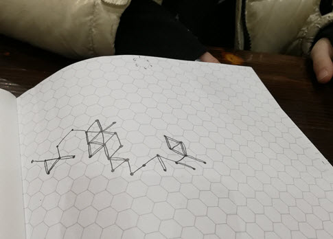
I was sitting in a bagel shop on Saturday with my 9 year old daughter. We had brought along hexagonal graph paper and a six sided die. We decided that we would choose a hexagon in the middle of the page and then roll the die to determine a direction:
1 up (North)
2 diagonal to the upper right (Northeast)
3 diagonal to the lower right (Southeast)
4 down (South)
5 diagonal to the lower left (Southwest)
6 diagonal to the upper left (Northwest)
Our first roll was a six so we drew a line to the hexagon northwest of where we started. That was the first “step.”
After a few rolls we found ourselves coming back along a path we had gone down before. We decided to draw a second line close to the first in those cases.
We did this about 50 times. The results are pictured above, along with kid hands for scale.
I sent the picture to my friend and serial co-author Jake Hofman because he likes a good kid’s science project and has a mental association for everything in applied math. He wrote “time for some Brownian motion?” and sent a talk he’d given a decade ago at a high school which taught me all kind of stuff I didn’t realize connecting random walks to Brownian motion, Einstein, the existence of atoms and binomial pricing trees in finance. (I was especially embarrassed not to have mentally connected random walks to binomial pricing because I had a slide on that in my job talk years ago and because it is the method we used in an early distribution builder paper.)
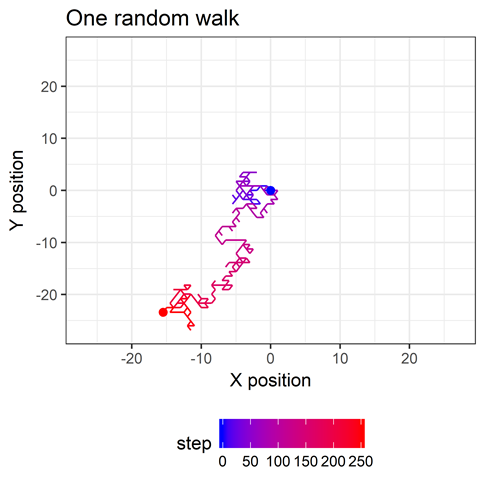
Back at home Jake did some simulations on random walks in one dimension (in which you just go forward or backward with equal probability) and sent them to me. Next, I did the same with hexagonal random walks (code at the end of this post). Here’s an image of one random walk on a hexagonal field.
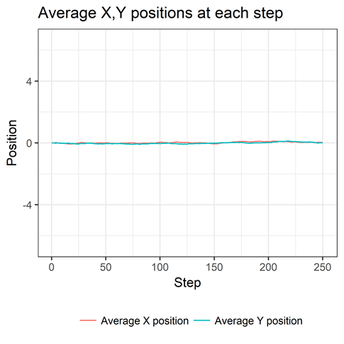
I simulated 5000 random walks of 250 steps, starting at the point 0,0. The average X and Y position is 0 at each step, as shown here.
This might seem strange at first. But think about many walks of just one step. The number of one-step journeys in which your X position is increased a certain amount will be matched, in expectation, by an equal number of one-step journeys in which your X position is decreased by the same amount. Your average X position is thus 0 at the first step. Same is true for Y. The logic scales when you take two or more steps and that’s why we see the flat lines we do.
If you think about this wrongheadedly you’d think you weren’t getting anywhere. But of course you are. Let’s look at your average distance from the starting point at each step (below).
The longer you walk, the more distant from the starting point you tend to be. Because distances are positive, the average of those distances is positive. We say you “tend to” move away from the origin at each step, because that is what happens on average over many trips. At any given step on any given trip, you could move towards or away from the starting point with equal probability. This is deep stuff.
Speaking of deep stuff, you might notice that the relationship is pretty. Let’s zoom in.
The dashed line is the square root of the number of steps. It’s interesting to note that this square root relationship happens in a one-dimensional random walk as well. There’s a good explanation of it in this document. As Jake put it, it’s as if the average walk is covered by a circular plate whose area grows linearly with the number of steps. (Why linearly? Because area of a circle is proportional to its radius squared. Since the radius grows as the square root of the number of steps, the radius squared is linear in the number of steps)
(*) As a sidenote, I was at first seeing something that grew more slowly than the square root and couldn’t figure out what the relationship was. It turns out that the square root relationship holds for the root mean squared distance (the mean of the squared distances) and I had been looking at the mean Euclidean distance. It’s a useful reminder that the term “average” has quite a few definitions. “Average” is a useful term for getting the gist across, but can lead to some confusion.
Speaking of gists, here’s the R code. Thanks to @hadleywickham for creating the tidyverse and making everything awesome.
RCODE


