FAMILIARITY-LIKING EFFECTS VIA CAPTCHAS

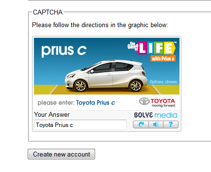
Decision Science News was creating a new account online and had to fill out the above-pictured CAPTCHA (*) to proceed. It’s an ad and a CAPTCHA in one. It gets people to spend time and effort typing the name of the brand. [If you don’t know what a CAPTCHA is see Wikipedia, or the Official CAPTCHA Site]
That time and effort should serve the advertiser well.
Cognitive psychologists know that the longer people spend processing a thing the more likely they are to remember it. By getting you to type the name of the brand, you become more likely to remember it, which is what advertisers want.
But this manipulation does double duty. Psychologists have also uncovered the familiarity-liking effect in which repeated stimuli (e.g. songs) become liked simply for being familiar. These studies randomly assign people to various stimuli, repeat the stimuli over time, and measure liking, which tends to increase. Each subsequent impression of an ad has this effect on you, but some ad impressions go unnoticed. By getting you to type the name of the brand, you are pretty sure to notice it. [Another thing that determines whether people notice ads is the amount of time they are in view, see our recent papers on this here and here].
What’s next? Will they go after the frequency-validity effect, by which familiar statements are judged as more likely to be true? If so, the CAPTCHAs of the future will ask you to type things like “I’m going to buy a Prius C right away!”
REFERENCES
Arkes, H. R., Hackett, C. and Boehm, L. (1989), The generality of the relation between familiarity and judged validity. Journal of Behavioral Decision Making, 2, 81–94.
Bornstein, Robert F. (1989) Exposure and affect: Overview and meta-analysis of research, 1968–1987. Psychological Bulletin, 106(2), 265-289.
Hintzman, Douglas L. and Richard A. Block (1971). Retition and memory: Evidence for a multiple-trace hypothesis. Journal of Experimental Psychology, 88(3), 297-306.
(*) One of the inventors of the CAPTCHA (the original one, not this manipulative version) is John Langford, a colleague of mine at Yahoo Research.
Filed in
Ideas
 Subscribe
 to Decision Science News by Email (one email per week, easy unsubscribe)
STRANGE WORD IN FRONT PAGE HEADLINES OF TWO NATIONAL NEWSPAPERS ON SAME DAY

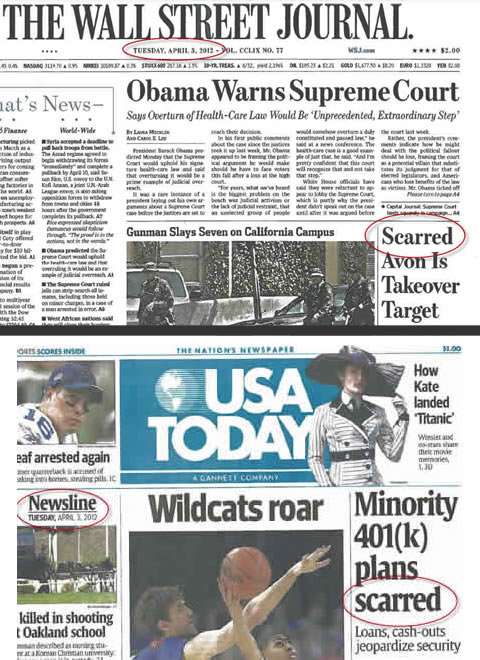
A friend of Decision Science News awoke in a hotel on April 3rd of this year and found two newspapers outside the door. The Wall Street Journal used the word “scarred” in its front page headline, which was weird enough, but all was made far weirder by the USA Today, which used the same word, also in a front page headline, also above the fold, on the same day.
We could overfit and say that “scarred” is the hot buzzword of 2012, or underfit and act as though there’s nothing to this at all, but instead we’ll just put it out there.
Scarred. Consider it out there.
SOCIETY FOR JUDGMENT AND DECISION MAKING NEWSLETTER

Just a reminder that the quarterly Society for Judgment and Decision Making newsletter can be downloaded from the SJDM site:
http://sjdm.org/newsletters/
It features jobs, conferences, announcements, and more.
Enjoy!
Decision Science News / SJDM Newsletter Editor
GLOBAL WEATHER DATA SUPERIMPOSED ON MAPS

At DSN, we’ve been playing a bit with FetchClimate Explorer from Microsoft Research. It lets one define regions of the globe over which it superimposes spatial and time series data concerning temperature, precipitation, sunlight, and, pictured above, wind speed.
See a demo of FetchClimate in this video, starting at 22:45.
The data (graphed above, larger image here) mesh with our experience living in Chicago that the “windy city” is not really that windy. Yes, Chicago is in a part of the country that is windier than average, but Kansas makes it look calm. Furthermore, New York City and Long Island are windier than Chicago, but nobody goes “OMG! How can you stand that wind?” when you say that you live there.
Average Wind Speed (meters / second)
- Chicago 4.92
- New York, NY 5.01
- Milwaukee, WI 5.03
- Casper, WY 5.5
- Rochester, MN 5.5
- Amarillo, TX 6.12
- Dodge City, KS 6.25
And a little wind is a good thing. Houston, TX (wind speed 4.11 m/s) would love a bit of air movement during its stifling summers. They say the phrase “windy city” has not to do with high winds or the hot air of politicians, but rather stems from an Chicago tourism slogan promoting the delightful summer breezes in the days before air conditioning.
MENTALLY MULTIPLY NUMBERS

If the numbers are both even or both odd
1. Learn how to square numbers in your head from our earlier post
2. Take the midpoint of the two numbers and square it. For example, if the numbers are 18 and 22, the midpoint is 20, which squared is 400
3. Square the difference between the midpoint and one of the original numbers. For example, the difference between 20 (midpoint number) and 18 (original number) is 2, which squared is 4.
4. Subtract step three from step two. 400 – 4 = 396. Done!
In general, (a + b) * (a -b) = a^2 – b^2. The trick is thinking of the two original numbers as (a+b) and (a-b) which are equally distant from a midpoint a.
If one number is even and the other odd
1. Round one number down or up so that both are even or both are odd. Apply the above method. Do one addition or subtraction to correct for the rounding. For example, think of 18*23 as 18*22 (which we solved above) plus 18.
Grab some pairs of numbers from the grid and try it. You may just like it!
P.S. Andrew Gelman: This is why you’d want to square numbers in your head.
Photo credit: http://www.flickr.com/photos/matthew-h/5579739816
Filed in
Books
 Subscribe
 to Decision Science News by Email (one email per week, easy unsubscribe)
Filed in
Conferences
 Subscribe
 to Decision Science News by Email (one email per week, easy unsubscribe)
ASSOCIATION FOR CONSUMER RESEARCH CONFERENCE, DEADLINE MARCH 19, 2012

CALL FOR PAPERS
Association for Consumer Research North American Conference
October 4-7, 2012, Vancouver, BC, Canada
Location: Sheraton Wall Centre Hotel
Conference Co-chairs:
Zeynep Gurhan-Can
Cele Otnes
Rui (Juliet) Zhu
Please address all inquiries regarding the information below to the
dedicated ACR email address:
acr2012@umn.edu
Conference website: http://www.acrweb.org/acr/Public/index.aspx
Important ACR 2012 Conference Deadlines:
Monday, March 19, 5 p.m. Central Standard Time: submission
deadline for all conference tracks except the Film Festival.
The 2012 North American Conference of the Association for Consumer
Research will be held at the Sheraton Wall Centre Hotel from
Thursday, October 4 through Sunday, October 7, 2012. The theme of
ACR 2012 is “Appreciating Diversity.” This theme is especially
appropriate for ACR Vancouver for at least two reasons. First, we want
the conference to acknowledge, capture and celebrate the explosion of
topics and research methods that has occurred in consumer research
in recent years. The co-chairs and track chairs will seek to highlight
scholarship that contributes to diversity in terms of innovative topics,
adds to knowledge in established areas in unheralded ways, embraces
diverse research applications and a wide array of consumers, and
contributes to inclusiveness in our field. Second, the theme is fitting
because of the progressive approach by our conference city,
Vancouver, to embrace diversity on multiple fronts. Not only is the city
varied in its population and economic base, but it also offers a
breathtaking array of experiences rooted in its geography and its
culture.
A pre-conference Doctoral Symposium will be held on Thursday, Oct. 4
(co-chaired by Jennifer Argo, University of Alberta and Amna Kirmani,
University of Maryland). The conference opens with a reception on
Thursday evening. The conference program on Friday and Saturday
will include Competitive Paper sessions, Special sessions, Roundtable
discussions, Poster sessions, and the Film Festival. A Gala Reception
will be held Saturday evening.
Filed in
Jobs
 Subscribe
 to Decision Science News by Email (one email per week, easy unsubscribe)
SOCIAL PSYCHOLOGY OPENINGS AT TILBURG SCHOOL OF SOCIAL AND BEHAVIORAL SCIENCES

Tilburg University is a modern, specialized university. The teaching and research of the Tilburg School of Social and Behavioral Sciences are organized around the themes of Health, Organization, and Relations between State, Citizen, and Society. The School’s inspiring working environment challenges its workers to realize their ambitions; involvement and cooperation are essential to achieve this.
The Department of Social Psychology of Tilburg University consists of a vibrant mix of people interested in Social, Economic and Work and Organisational psychology. The Department actively strives to create and maintain an intellectually stimulating and productive group, advancing our knowledge on a variety of social, economic and work and organisational topics, while at the same time contributing to the development of effective practices for organisations and society. The research of the department is highly recognized, both nationally and internationally.
We have vacancies (full-time, F/M) for:
Two Assistant Professors in Social Psychology (Tenure Track)
One Assistant Professor in Social Psychology (Fixed Term, 3 years)
Members of the Department of Social Psychology supervise students, teach a variety of modules at both Bachelors’ and Masters’ level, including the two-year Research Master. The global research program of the Department of Social Psychology is centered around Social Decision Making. Department members also participate in the interdisciplinary research institute TIBER, the Tilburg Institute for Behavioral Economics Research, which is devoted to studying choice and decision making from an interdisciplinary perspective.
Tasks
You will work in the area of Social Psychology, Economic Psychology or Work & Organisational Psychology. You are expected to:
- conduct empirical research fitting within the global research program of the Department
- write and publish articles in international peer-reviewed journals
- teach courses (in Dutch or English) offered by the department on the BSc and MSc level
- supervise individual students at BSc and MSc level
Qualifications
We expect candidates to:
- have a PhD degree in Psychology or in a related area
- be a passionate researcher/teacher
- have high quality publications in international, peer-reviewed scientific
- have experience and affinity with teaching in the area of Social Psychology, Economic Psychology, and/or Work and Organizational Psychology
- have good command of English at an academic level
Terms of employment
We offer one fixed term and two tenure track positions. Tenure track positions consist of a four-year contract with the possibility of tenure thereafter. The fixed term contract is for three years. The salary for the position of an Assistant Professor on a full-time basis ranges between € 3195,- and € 4374,- per month (for a full-time appointment, various allowances are not included) based on scale 11 of the Collective Labour Agreement (CAO) Dutch Universities. Researchers from outside the Netherlands may qualify for a tax-free allowance equal to 30% of their taxable salary. The university can apply for such an allowance on their behalf. The university offers very good fringe benefits, such as an options model for terms and conditions of employment and excellent reimbursement of moving expenses.
Applications and information
Additional information about Tilburg University and the Department of Social Psychology can be retrieved from: www.uvt.nl. Specific information about the vacancy can be obtained from Ilja van Beest, Professor of Social Psychology, telephone +31134662472, email: I.VanBeest@uvt.nl, or from Marcel Zeelenberg, Professor of Economic Psychology & Department Head, telephone +31134668381, email: Marcel@uvt.nl.
Applications, including a curriculum vitae, a letter of motivation, and two recent (or forthcoming) publications should be send, before March 30, 2012 only by the link below to drs. J.H. Dieteren, Managing Director Tilburg School of Social and Behavioral Sciences, Tilburg University, The Netherlands.
http://erec.uvt.nl/vacancy?inc=UVT-EXT-2012-0076
MENTALLY MULTIPLY NUMBERS BY THEMSELVES

Babbage’s Difference Engine is fueled by squares
Even in the age of ubiquitous computing, its usually faster to do a simple operation like squaring a number in your head as opposed to doing it on paper or firing up R. Everyday decision making in science needs to happen in a fast and frugal manner. Assuming you know your multiplication tables up to 10×10, here’s how to compute the squares of numbers up to 100 in your noggin (and beyond if you are willing to bootstrap).
A. If the number ends in 0, chop off the 0s, square what is left, and put back two 0s for each one you knocked off. Examples:
- 50: chopping off the zero gives 5, squaring that gives 25, replacing the 0 with two 0s gives 2500
- 100: chopping off the zero gives 1, squaring that gives 1, replacing each chopped 0 with two gives 10,000
B. If the number ends in 5, chop of the five, take what is left and multiply it by the next highest number, stick 25 on the end Examples:
- 35: chopping off the 5 gives 3, multiplying what’s left (3) by the next highest number (4) gives 12, sticking 25 on the end gives 1225
- 95: chopping off the 5 gives 9, multiplying what’s left (9) that by the next highest number (10) gives 90, sticking 25 on the end gives 9025
C. If the number is 1 greater than a number that ends in 5 or 0, first square the number ending in 5 or 0, as above, then add to this the number ending in 5 or 0 and the number. Examples:
- 51: 51 is one greater than 50, the square of which we know from above is 2500. To this we add the number ending in 5 or 0 (50) and the number (51). 2500 + 50 + 51 = 2601
- 36: 36 is one greater than 35, the square of which we know from above is 1225. To this we add the number ending in 5 or 0 (35) and the number (36). 1225 + 35 + 36 = 1296
If the number is 1 less than a number that ends in 5 or 0, first square the number ending in 5 or 0, as above, then subtract from this the number ending in 5 or 0 and the number. Examples:
- 49: 49 is one less than 50, the square of which we know from above is 2500. From this we subtract the number ending in 5 or 0 (50) and the number (49). 2500 – 50 – 49 = 2401
- 34: 34 is one less than 35, the square of which we know from above is 1225. From this we subtract the number ending in 5 or 0 (35) and the number (34). 1225 – 35 – 34 = 1156
D. If the number is 2 greater than a number that ends in 5 or 0, first square the number ending in 5 or 0, as above, then add to this four times the number that is 1 greater than the number ending in 5 or 0. Examples:
- 52: 52 is two greater than 50, the square of which we know from above is 2500. To this we add four times the number that is 1 greater than the number ending in 5 or 0 (51). 2500 + 4 * 51 = 2704
- 37: 37 is two greater than 35, the square of which we know from above is 1225. To this we add four times the number that is 1 greater than the number ending in 5 or 0 (36). 1225 + 4 * 36 = 1369
If the number is 2 less than a number that ends in 5 or 0, first square the number ending in 5 or 0, as above, then subtract from this four times the number that is 1 less than the number ending in 5 or 0. Examples:
- 48: 48 is two less than 50, the square of which we know from above is 2500. From this we subtract four times the number that is 1 less than the number ending in 5 or 0 (49). 2500 – 4 * 49 = 2304
- 33: 33 is two less than 35, the square of which we know from above is 1225. From this we subtract four times the number that is 1 less than the number ending in 5 or 0 (34). 1225 – 4 * 34 = 1089
Since every number is either 1 or 2 greater or less than a number ending in 0 or 5, we are done.
Happy squaring!
Proof of C: First part: (N+1)^2=N^2+N+(N+1), Second part (N-1)^2=N^2-N-N+1=N^2-N-(N-1)
Proof of D: First part: (N+2)^2=N^2+4N+4=N^2+4(N+1), Second part (N-2)^2=N^2-4N+4=N^2-4(N-1)
Photo credit: http://www.flickr.com/photos/mrgiles/325903759/
Filed in
Ideas
 Subscribe
 to Decision Science News by Email (one email per week, easy unsubscribe)
SIMPLE RULES FOR DIETING

This is what we’ve figured out from our experiments.
- Live 1.5 miles from your workplace. It’s too short to drive, so you just walk.
- Stop deciding what to eat for a week. Worked for us.
- Eat the same thing for breakfast every day (source: Brian Wansink). He’s found correlational evidence for this.
- Use small plates (source: Brian Wansink). Experiments show that this affects consumption (at least during the experiment).
- Put money on the line (source: Daniel Reeves). With enough money on the line, it seems like it would just have to work. Beeminder.com is our nerdy favorite. Stickk.com is also good
- Weigh your food with a gram scale. Pouring 20 grams less cereal in the AM makes a difference. Also, a gram scale is the key to making the perfect pot of coffee. We have this one
 , among others.
- Learn to estimate calories. We’re making a video game of this, but fitday.com is a fun place to start.
- Don’t eat more than 500 calories at a time. You’re probably not hungry 15 minutes after stopping.
- Round the calories in fruits and vegetables down to zero. WeightWatchers has apparently moved to this in their new point system. It’s obviously wrong, but it works.
photo credit:http://www.flickr.com/photos/puuikibeach/4470122675
 Subscribe to Decision Science News by Email (one email per week, easy unsubscribe)
