Decision Science News

HANDY COMPUTER PROGRAMS FOR TURNING NUMBERS INTO MEMORABLE WORDS

Two posts ago we showed you the digit sound system for remembering numbers. This week we provide two Python programs (and one R program) to help you create mnemonics.

w2num.py – converts every word in the English language to a number
find.py – takes a longish number and gives you words that when put together translate into that number using the digit-sound system.

If you are not a programmer, or if you are lazy, you can get to the chase and just download the relevant outupt files here

wordNum.txt – every word in English translated into a number using the digit-sound system
numWords.txt – All the English words that translate into a given number

However, you have a long number that you want to make a mnemonic for, you’re better off using find.py or find.R below to find mnemonics. These handy programs break up long numbers into shorter ones which do have mnemonics.

NOTES:
These programs use phonetics (not spelling) to make the mnemonics. Read the small print on Jap Murre’s site to see why “letter” is 514 and not 5114 and why “ing” is 27. Thanks to Daniel Reeves for convincing discussions on the merits of using a purely phonetic system.

As usual, we’re open for suggestions on how to improve these programs … they’re both kind of slapdash jobs.

##w2num.py##
Prerequisites: You need to save a couple of wordlists locally. In particular
1) You need to save a copy of http://bit.ly/xz8YIC
as cmudict-0.4.scm. This is a mapping from words in English to phonemes.
2) You need to save a copy of http://scrapmaker.com/data/wordlists/twelve-dicts/2of12inf.txt
as wordlist.txt. This is a list of reasonably common English words (b/c some of the words in cmudict are too rare to be useful).
3) Put cmudict-0.4.scm and wordlist.txt in the same directory as
w2num.py and then do
python w2num.py > wordNum.txt
to generate the number corresponding to every English word. (If in the future these URLs break, just search around for copies of cmudict-0.4.scm and 2of12inf.txt …there are many copies of these dictionaries around.)

##find.py##
This is the program you use when you have a longish number and you want to find words that encode it. It uses recursive ™ technology to break up numbers a few different ways to increase your chances of finding a mnemonic you like.
Prerequisite: You must have created wordNum.txt (by running python w2num.py > wordNum.txt) in the previous step and saved it to the same directory as this program before running.
To turn a number like 8675309 into words do
python find.py 8675309

Lastly, for kicks I wrote a slightly dumber version of find.py in R. It lacks the cool “rec3” method of finding mnemonics but it gets the job done.

##find.R##
Same as find.py
Prerequisite: same as find.py
To turn a number like 8675309 into words change the variable mstr to ‘8675309’ and run the program.

SOCIETY FOR JUDGMENT AND DECISION MAKING NEWSLETTER

Just a reminder that the Quarterly Society for Judgment and Decision Making newsletter can be downloaded from the SJDM site:

http://sjdm.org/newsletters/

Enjoy!

RESOLVE TO MEMORIZE NUMBERS WITH THE DIGIT-SOUND METHOD

At Decision Science News, we have all kinds of numbers memorized: IP addresses, passport numbers, phone numbers, bank account numbers, logarithms, etc. Once you have stuff like this memorized, you’ll  realize how much of a hassle it was to look all this stuff up all the time. Besides, it’s fun.

But how is it done?

It is done with the digit-sound method, which we learned from Professor Jaap Murre’s neuroMod site at the University of Amsterdam. According to Murre, this amazing method traces back to 1648!

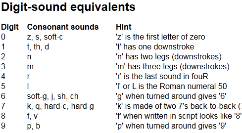
You associate a digit with a sound or sounds like this

0 z, s, soft-c ‘z’ is the first letter of zero
1 t, th, d ‘t’ has one downstroke
2 n ‘n’ has two legs (downstrokes)
3 m ‘m’ has three legs (downstrokes)
4 r ‘r’ is the last sound in fouR
5 l ‘l’ or L is the Roman numeral 50
6 soft-g, j, sh, ch ‘g’ when turned around gives ‘6’
7 k, q, hard-c, hard-g ‘k’ is made of two 7’s back-to-back
8 f, v ‘f’ when written in script looks like ‘8’
9 p, b ‘p’ when turned around gives ‘9’

Then, when you want to remember a number, you simply replace the digits with sounds and try to make a vivid phrase. Any vowels or sounds not included in the chart are ignored when you are reading back the phrase. For example, suppose you want to memorize Jenny’s phone number: 867-5309.

Here’s how we might do it:

• Change 867 to sounds, such as “f”, “sh” and “k”
• Change 5309 to sounds, such as “l”, “m”, “s” and “b”
• Now insert vowels and letters not on the chart in order to generate a vivid phrase from those sounds.

We came up with the following dialog involving a parent and child at the dinner table:

–“Fish, ok?”
–“Lame! *sob*”

In this mini play, we have “f”, “sh”, “k” “l”, “m”, “s” and “b” in order, and can easily reconstruct 867-5309. Remember, when reading it back, you ignore all vowels and letters that aren’t in the chart.

The only start-up cost is memorizing the chart, but that’s not hard. There’s even a training tool so you can practice until you have the associations down pat.

Of course, since there can be a few possible sounds for each letter, you need to play around a bit to find a phrase that works for you. To generate possibilities for long numbers, we’ve written the following python script.

NOTE 1: In this code, we’ve simplified the digit-sound method to include fewer letters since we always get confused with hard vs soft letters. We find the simplified method works just fine for us.
NOTE 2: This code is written in a hackish, randomized way that generates wasteful dupes. However, we don’t care since it doesn’t output the dupes, it runs super fast, and if you have a huge number of possibilities, you don’t want to see them all anyway. That said, if people have better implementations, we’re open for suggestions. Thanks to Dan Reeves for tightening up the code a bit!
NOTE 3: You can take the output of this program and hunt for words that fit the patterns with a linux call like this.
grep -E ‘^l[aieouy]*m[aieouy]*n[aeiouy]*$’ wordlist.txt
Where you are looking for words that match “l”, “m”, “n” and wordlist.txt is a list of words, one per line. You can find many wordlists here.

#Usage. Save this file as generate.py
#Then to use, do generate.py 867 (if 867 is the number for
#which you want to generate letters)
from cStringIO import StringIO
import random
from sys import argv
from time import strftime
mstr=str(argv[1])
def genString():
        numsounds = [['s','z'], ['t','th','d'],['n'],['m'],['r'],\
['l'],['j','ch','sh',],['k','q'],['f','v'],['p','b']]
        return [random.choice(numsounds[int(i)]) for i in mstr]
i=0
myDict={}
while i<10000:
        astr=' '.join(genString())
        if not myDict.has_key(astr):
                myDict[astr]=1
                print '%-20s ==> %2d : %20s' % \
(astr,i,strftime("%Y-%m-%d %H:%M:%S"))
        i=i+1

Photo credit: http://memory.uva.nl/memimprovement/eng/phon_peg_1.htm

LEARN HOW TO IMPORT WORLD BANK DATA AND INVEST IN THE WHOLE WORLD

Click to enlarge
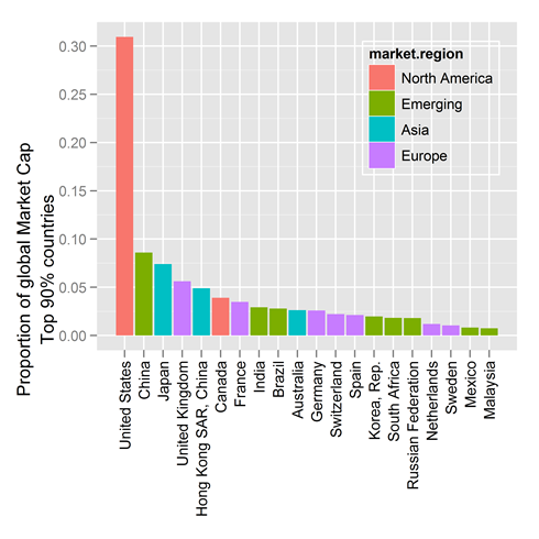
The market cap of the countries comprising 90% of the world’s market cap (end 2010)

A famous finance professor once told us that good diversification meant holding everything in the world. Fine, but in what proportion?

Suppose you could invest in every country in the world. How much would you invest in each? In a market-capitalization weighted index, you’d invest in each country in proportion to the market value of its investments (its “market capitalization”). As seen above, the market-capitalization of the USA is about 30%, which would suggest investing 30% of one’s portfolio in the USA. Similarly, one would put 8% in China, and so on. All this data was pulled from the World Bank, and at the end of this post we’ll show you how we did it.

What makes life easy is that economists have grouped countries into regions and the market caps of each can be computed by summing the market caps of the constituent countries. See this MSCI page for the manner in which we’ve categorized countries in this post:

North America: USA, Canada
Emerging: Brazil, Chile, China, Colombia, Czech Republic, Egypt, Hungary, India, Indonesia, Korea, Malaysia, Mexico, Morocco, Peru, Philippines, Poland, Russia, South Africa, Taiwan, Thailand, Turkey
Asia: Japan, Australia, Hong Kong, New Zealand, Singapore
Europe: Austria, Belgium, Denmark, Finland, France, Germany, Greece, Ireland, Italy, Netherlands, Norway, Portugal, Spain, Sweden, Switzerland, United Kingdom
Other: Everybody else in the world

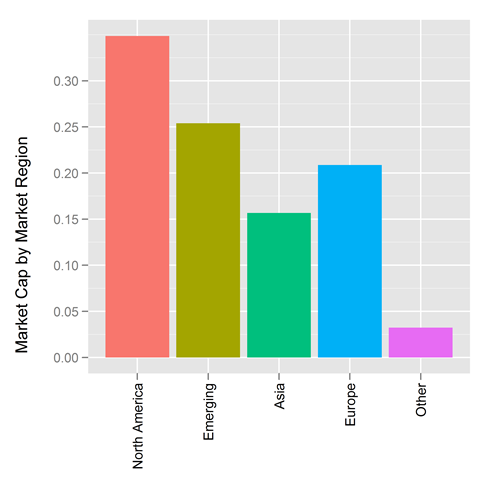
What makes life easier still is that one can purchase ETFs that work like indices tracking the various regions of the world. For example at Vangard one can purchase

• Vanguard Total Stock Market ETF (Ticker VTI), which basically covers North America
• Vanguard MSCI Emerging Marketing ETF (Ticker VWO), which covers emerging markets
• Vanguard MSCI Pacific ETF (Ticker VPL), which covers Asia (minus the Asian emerging markets countries)
• Vanguard MSCI Europe ETF (Ticker VGK), which covers Europe

What makes life a bit more complicated is that not everybody agrees on market-cap weighting. Some favor Gross Domestic Product (GDP) weighting for the reasons given at this MSCI page.

• GDP figures tend to be more stable over time compared to equity markets’ performance-related peaks and troughs
• GDP weighted asset allocation tends to have higher exposure to countries with above average economic growth, such as emerging markets
• GDP weighted indices may underweight countries with relatively high valuation, compared to market-cap weight indices

Here are the countries that make up 90% of the world’s GDP:

Click to enlarge
The GDP of the countries comprising 90% of the world’s GDP (end 2010)

Because we love you, we’ve also computed how the classic market regions compare to one another in terms of GDP

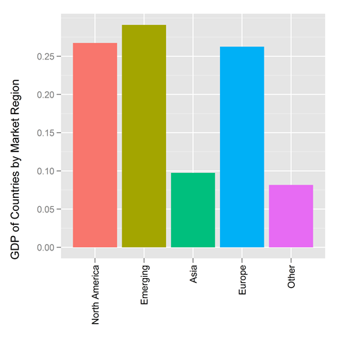
If you track changes in market cap from month to month as we do, you’ll appreciate the stability that GDP weighting provides. For example, the market cap data in this post, from 2010, is already way out of date.

So, weight by market cap, or weight by GDP, or do what we do and weight by the average of market cap and GDP, but don’t wait to diversify your portfolio outside of a handful of investments you happen to own. Invest in the world.

For those who love R and who want to learn how to pull down World Bank data, the code is provided here. I got started with this by borrowing code from this very helpful blog post by Markus Gesmann and tip my hat to its author. Thanks also to Hadley for writing ggplot2 (and for visiting us at Yahoo the other week. And thanks to Yihui Xie for his code formatter.

R CODE

library(ggplot2)
library(car)
library(RJSONIO)
ftse=read.delim("201112_FTSE_Market_Caps.tsv",sep="\t")
##See www.msci.com/products/indices/tools/index.html
##Emerging::Brazil, Chile, China, Colombia, Czech Republic, Egypt, Hungary,
#India, Indonesia, Korea, Malaysia, Mexico, Morocco, Peru, Philippines,
#Poland, Russia, South Africa, Taiwan, Thailand, Turkey
##Europe::Austria, Belgium, Denmark, Finland, France, Germany, Greece, Ireland, Italy,
#Netherlands, Norway, Portugal, Spain, Sweden, Switzerland, United Kingdom
##Asia::Japan, Australia, Hong Kong, New Zealand, Singapore
recodestring=" c('USA','CAN')='North America';
c('BRA','CHL','CHN','COL','CZE','EGY','HUN','IND','IDN','KOR','MYS','MEX','MAR','PER','PHL','POL',
'RUS','ZAF','TWN','THA','TUR')= 'Emerging';
c('AUT','BEL','DNK','FIN','FRA','DEU','GRC','IRL','ITA',
'NLD','NOR','PRT','ESP','SWE','CHE','GBR')= 'Europe';
c('JPN','AUS','HKG','NZL','SGP')= 'Asia';
else='Other'"
#How much of the world do we want to consider (to keep graphs manageable)
CUTOFF=.9
#Some code from internet to read world bank data. Adapted from
#http://www.r-bloggers.com/accessing-and-plotting-world-bank-data-with-r/
#See also http://data.worldbank.org/indicator/NY.GDP.MKTP.CD
getWorldBankData = function(id='NY.GDP.MKTP.CD', date='2010:2011',
value="value", per.page=12000){
require(RJSONIO)
url = paste("http://api.worldbank.org/countries/all/indicators/", id,
"?date=", date, "&format=json&per_page=", per.page,
sep="")
wbData = fromJSON(url)[[2]]
wbData = data.frame(
year = as.numeric(sapply(wbData, "[[", "date")),
value = as.numeric(sapply(wbData, function(x)
ifelse(is.null(x[["value"]]),NA, x[["value"]]))),
country.name = sapply(wbData, function(x) x[["country"]]['value']),
country.id = sapply(wbData, function(x) x[["country"]]['id'])
)
names(wbData)[2] = value
return(wbData)
}
getWorldBankCountries = function(){
require(RJSONIO)
wbCountries =
fromJSON("http://api.worldbank.org/countries?per_page=12000&format=json")
wbCountries = data.frame(t(sapply(wbCountries[[2]], unlist)))
levels(wbCountries$region.value) = gsub("\\(all income levels\\)",
"", levels(wbCountries$region.value))
return(wbCountries)
}
### Get the most recent year with data
curryear = as.numeric(format(Sys.Date(), "%Y"))
years = paste("2010:", curryear, sep="")
##Get GDP for the countries (GDP in Current US Dollars)
GDP = getWorldBankData(id='NY.GDP.MKTP.CD',
date=years,
value="gdp")
#If a year has > 60 NAs it is not ready
while( sum(is.na(subset(GDP,year==curryear)$gdp)) > 60 )
{curryear=curryear-1}
#Keep just the most current year
GDP=subset(GDP,year==curryear);
## Get country mappings
wbCountries = getWorldBankCountries()
## Add regional information
GDP = merge(GDP, wbCountries[c("iso2Code", "region.value", "id")],
by.x="country.id", by.y="iso2Code")
## Filter out the aggregates, NAs, and irrelevant columns
GDP = subset(GDP, !region.value %in% "Aggregates" & !is.na(gdp))
GDP=GDP[,c('year','gdp','country.name','region.value','id')]
GDP=GDP[order(-1*GDP[,2]),]
GDP$prop=with(GDP,gdp/sum(gdp))
GDP$cumsum=cumsum(GDP$gdp)
GDP$cumprop=with(GDP,cumsum(gdp)/sum(gdp))
GDP$market.region=recode(GDP$id,recodestring)
resize.win <- function(Width=6, Height=6) { plot.new() dev.off(); #dev.new(width=6, height=6) windows(record=TRUE, width=Width, height=Height) } slice=max(which(GDP$cumprop<=CUTOFF)) smGDP=GDP[1:slice,] smGDP$country.name=factor(smGDP$country.name,levels=unique(smGDP$country.name)) smGDP$region.value=factor(smGDP$region.value,levels=unique(smGDP$region.value)) smGDP$market.region=factor(smGDP$market.region,levels=unique(smGDP$market.region)) g=ggplot(smGDP,aes(x=as.factor(country.name),y=prop)) g=g+geom_bar(aes(fill=market.region)) g=g+opts(axis.text.x=theme_text(angle=90, hjust=1))+xlab(NULL)+ ylab( paste("Proportion of global GDP\nTop ",CUTOFF*100,"% countries",sep="")) g=g+opts(legend.position=c(.8,.8)) resize.win(5,5) #might have to run this twice to get it to shift from the default window g ggsave("GDPbyCountry.png",g,dpi=600) smGDPsum=ddply(GDP,.(market.region),function(x) {sum(x$gdp)}) smGDPsum$V1=smGDPsum$V1/sum(smGDPsum$V1) smGDPsum=smGDPsum[order(-1*smGDPsum[,2]),] smGDPsum$market.region=factor(smGDPsum$market.region,levels=c("North America","Emerging","Asia","Europe","Other")) g=ggplot(smGDPsum,aes(x=as.factor(market.region),y=V1)) g=g+geom_bar(aes(fill=market.region)) g=g+opts(axis.text.x=theme_text(angle=90, hjust=1))+xlab(NULL)+ylab("GDP of Countries by Market Region\n") g=g+opts(legend.position="none") resize.win(5,5) #might have to run this twice to get it to shift from the default window g ggsave("GDPbyRegion.png",g,dpi=600) ##Get Market Cap data from World Bank CM.MKT.LCAP.CD ### Get the most recent year with data curryear = as.numeric(format(Sys.Date(), "%Y")) years = paste("2010:", curryear, sep="") ##Get MarketCap for the countries (MCP in Current US Dollars) MCP = getWorldBankData(id='CM.MKT.LCAP.CD', date=years, value="mcp") #If a year has > 60 NAs it is not ready
while( sum(is.na(subset(MCP,year==curryear)$mcp)) > 150 )
{curryear=curryear-1}
#Keep just the most current year
MCP=subset(MCP,year==curryear);
## Add regional information
MCP=merge(MCP, wbCountries[c("iso2Code", "region.value", "id")],
by.x="country.id", by.y="iso2Code")
## Filter out the aggregates, NAs, and irrelevant columns
MCP = subset(MCP, !region.value %in% "Aggregates" & !is.na(mcp))
MCP=MCP[,c('year','mcp','country.name','region.value','id')]
MCP=MCP[order(-1*MCP[,2]),]
row.names(MCP)=NULL
MCP$prop=with(MCP,mcp/sum(mcp))
MCP$cumsum=cumsum(MCP$mcp)
MCP$cumprop=with(MCP,cumsum(mcp)/sum(mcp))
MCP$market.region=recode(MCP$id, recodestring)
slice=max(which(MCP$cumprop<=CUTOFF)) smMCP=MCP[1:slice,] smMCP$country.name=factor(smMCP$country.name,levels=unique(smMCP$country.name)) smMCP$region.value=factor(smMCP$region.value,levels=unique(smMCP$region.value)) smMCP$market.region=factor(smMCP$market.region,levels=unique(smMCP$market.region)) g=ggplot(smMCP,aes(x=as.factor(country.name),y=prop)) g=g+geom_bar(aes(fill=market.region)) g=g+opts(axis.text.x=theme_text(angle=90, hjust=1))+xlab(NULL)+ ylab( paste("Proportion of global Market Cap\nTop ",CUTOFF*100,"% countries",sep="")) g=g+opts(legend.position=c(.8,.8)) resize.win(5,5) #might have to run this twice to get it to shift from the default window g ggsave("MCPbyCountry.png",g,dpi=600) smMCPsum=ddply(MCP,.(market.region),function(x) {sum(x$mcp)}) smMCPsum$V1=smMCPsum$V1/sum(smMCPsum$V1) smMCPsum=smMCPsum[order(-1*smMCPsum[,2]),] smMCPsum$market.region=factor(smMCPsum$market.region,levels=c("North America","Emerging","Asia","Europe","Other")) g=ggplot(smMCPsum,aes(x=as.factor(market.region),y=V1)) g=g+geom_bar(aes(fill=market.region)) g=g+opts(axis.text.x=theme_text(angle=90, hjust=1))+xlab(NULL)+ylab("Market Cap by Market Region\n") g=g+opts(legend.position="none") resize.win(5,5) #might have to run this twice to get it to shift from the default window g ggsave("MCPbyRegion.png",g,dpi=600)

YOU CAN NEVER THINK UP ALL THE NON-SINISTER EXPLANATIONS FOR THAT FACT

This week, DSN suggests watching a couple videos.

First, this captivating Errol Morris short, The Umbrella Man, over at the New York Times.

Next, this clip of Sofitel Hotel security guards dancing (or is it hugging?) in a backroom shortly after their colleague reported a sexual assault by Dominique-Strauss Kahn. More videos here.

Lastly, the famous case of People vs. Collins.

A robbery was reported as having been carried out by an African-American man with a beard and mustache in the company of a blond Caucasian woman with a ponytail who escaped in a yellow convertible. A couple fitting that description, the Collinses, was picked up. Faulty mathematics were use to infer “that there could be but one chance in 12 million that defendants were innocent and that another equally distinctive couple actually committed the robbery.” (See the Wikipedia page for how they arrived at this). A computation later in the Supreme Court of California Decision (People v. Collins, 68, Cal.2d 334, 335 (Cal. 1968)) figures that even with the prosecutor’s assumptions:

we would derive probability of over 40 percent that the couple observed by the witnesses could be “duplicated” by at least one other equally distinctive inter-racial couple in the area, including a Negro with a beard and mustache, driving a partly yellow car in the company of a blonde with a ponytail. Thus the prosecution’s computations, far from establishing beyond a reasonable doubt that the Collinses were the couple described by the prosecution’s witnesses, imply a very substantial likelihood that the area contained more than one such couple, and that a couple other than the Collinses was the one observed at the scene of the robbery.

We close with the closing words of the umbrella man:

If you have any fact, which you think is really sinister … is really obviously a fact that can only point to some sinister underpinnings … hey forget it, man, because you can never on your own think up all the non-sinister perfectly valid explanations for that fact. A cautionary tale.

We’re not stating an opinion on guilt or innocence in the above cases. We’re just encouraging a bit of reflection on what “beyond a reasonable doubt” should mean.

ADDENDUM: A lighter take on correlation and causation.

Hat Tip to Mark Fasciano for the Umbrella man.

2012 BEHAVIORAL DECISION RESEARCH IN MANAGEMENT CONFERENCE

The Behavioral Decision Research in Management Conference is held biennially and brings together the best of behavioral research within, but not limited to, the areas of consumer behavior, organizational behavior, negotiation, managerial decision making, behavioral finance, experimental and behavioral economics, decision analysis, behavioral strategy, behavioral operations research, behavioral accounting, and medical and legal decision making.

The conference will hosted by the Leeds School of Business at the University of Colorado, Boulder June 27-29, 2012 at the St. Julien Hotel in Boulder, CO.

Inquiries about BDRM 2012 should be directed to bdrm2012inquiries@colorado.edu

Conference Website

Call for papers

Submit to the conference (Deadline Feb 10, 2012)

THE SAME EVENT DESCRIBED IN DIFFERENT-SOUNDING WAYS

We’ve written before about avoiding relative risk formats in communicating risks to the general public.

One issue is that subtle changes in terminology lead to vastly different figures. For example, imagine there are two coaches, A and B. When Coach A  is working, the team catches the ball 16 times per 100.  When Coach B is working, the team catches the ball 8 times per 100. Those are the facts. Now lets look at the range of numbers we can generate with relative risks from those facts.

• Going from Coach B to Coach A, the relative chance of catching the ball increases 100%. Let’s publish it in Science!
• Going from Coach A to Coach B, the relative chance of catching the ball drops 50%. Somebody call the newspaper!
• Going from Coach A to Coach B, the relative chance of dropping the ball increases 9.5%. Yawn
• Going from Coach B to Coach A, the relative chance of dropping the ball decreases 8.7%. Zzz….

After reading, many people will forget details such as whether the statistic was going from A to B or B to A,  whether it concerned catching or dropping, or what the sign was, leaving different people with different vague ideas that something in the set of -100%, -50%, -9.5%, -8.7%, 8.7%, 9.5%, 50%, 100% had something to do with coach quality.

We see here that relative risk formats can make a catch rate change from 16% to 8% look like a very different animal than a drop rate change from 84% to 92%. But they are not different animals, they are two ways of referring to the exact same event.

Don’t believe me? Without looking up, try to remember the relative change in drop rate going from Coach A to Coach B.

So. Is the best practice just to give two numbers, that is, tell the readers the catch rate went from 16% to 8%? Or to tell them that the drop rate went from 84% to 92%?

The problem is, even when avoiding relative risk formats, changes between small numbers just look bigger than changes between big numbers, even when the small numbers and the big numbers express the exact same event. That is, 8 vs 16 looks like a bigger deal than 92 vs 84.

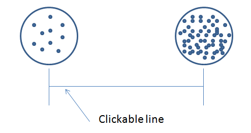
Here’s an experimental demonstration. Stanislas Dehaene and colleagues surveyed Mundurucu participants (in the Amazon) and Western participants (in the USA) on where they felt numbers lie on a scale from from 10-100. Specifically, participants had an interface like that pictured above, with 10 dots on the left and 100 dots on the right. They were then shown between 10 and 100 dots and asked to click on the line where they would fall.

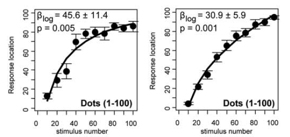
Data on the left are from the Mundurucu participants, those on the right from American participants.

Both the Amazonians and the US participants had negatively accelerated response curves. For instance, when shown 30 dots, the Mundurucu clicked the middle of the scale, and the Americans placed 40 dots in the middle of the scale. With such curves, differences between small numbers take up more space on the scale than equal differences between large numbers, which is why a rate change of 16 to 8 sounds like a bigger deal than a  rate change of 84 to 92. This is another instance in which people seem attuned to relative differences over and above absolute differences: the Weber-Fechner idea.

When expressing changes in probabilities, it makes us nervous that people can play games. They can choose between small numbers (here catch rates) and large numbers (drop rates) to play up or play down a point.  This post discusses how this can happen whether one uses relative risk calculations or simply provides before and after numbers. This is one reason we are fans of providing absolute changes in probability. Going from Coach A to Coach B, catches decreased 8 percentage points, which is to say drops increased by 8 percentage points. With this formulation, no matter how the thing is expressed, the only thing the forgetful can get wrong is the sign.

REFERENCES

Dehaene, Izard, Spelke, Pica. (2008). Log or Linear? Distinct Intuitions of the Number Scale in Western and Amazonian Indigene Cultures. Science, 320, pp 1217-1220.

Addition Is Useless, Multiplication Is King: Channeling Our Inner Logarithm

XKCD: Percentage Points

R CODE

options(digits=2)
CoachAcatch=16 # Coach 1 catch rate
CoachAdrop=100-CoachAcatch # Coach 1 drop rate
CoachBcatch=8 # Coach 2 catch rate
CoachBdrop=100-CoachBcatch # Coach 2 drop rate
#Going from Coach A to Coach B
sprintf("Relative risk of catching the ball: %.1f%%",(CoachBcatch-CoachAcatch)/CoachAcatch*100)
sprintf("Relative risk of dropping the ball: %.1f%%",(CoachBdrop-CoachAdrop)/CoachAdrop*100)
#Going from Coach B to Coach A
sprintf("Relative risk of catching the ball: %.1f%%",(CoachAcatch-CoachBcatch)/CoachBcatch*100)
sprintf("Relative risk of dropping the ball: %.1f%%",(CoachAdrop-CoachBdrop)/CoachBdrop*100)
#Going from Coach A to Coach B
sprintf("Absolute risk of catching the ball: %.1f%%",(CoachBcatch-CoachAcatch))
sprintf("Absolute risk of dropping the ball: %.1f%%",(CoachBdrop-CoachAdrop))
#Going from Coach B to Coach A
sprintf("Absolute risk of catching the ball: %.1f%%",(CoachAcatch-CoachBcatch))
sprintf("Absolute risk of dropping the ball: %.1f%%",(CoachAdrop-CoachBdrop))


SOCIETY FOR CONSUMER PSYCHOLOGY FIRST INTERNATIONAL CONFERENCE, FLORENCE ITALY

SOCIETY FOR CONSUMER PSYCHOLOGY
First International Conference
La Pietra Conference Center, Florence, Italy
June 29-July 1, 2012

SUBMISSION DEADLINE: Thursday, December 15, 2011

Conference Co-chairs:
Simona Botti, London Business School
Vicki Morwitz, New York University
Stefano Puntoni, Erasmus University

The aim of this conference is to foster the exchange of innovative theories and findings among psychologists and consumer researchers coming from different parts of the world. The small size of the conference (max120 attendees), the intimate Villa La Pietra location, the stunning Florence background, and the inspiring keynote speeches from Anne Maass (University of Padova) and Peter Gollwitzer (New York University), should facilitate idea generation and new collaborations.

Conference Web Site

Call For Papers

ABSTRACT SUBMISSION DEADLINE: DECEMBER 15, 2011

Hi Folks – This year BDRM will back back to back with with Boulder Summer Conference on Consumer Financial Decision Making. What an excellent reason to attend both!

What: 2012 Boulder Summer Conference on Consumer Financial Decision Making
When: June 24-26, 2012
Where St. Julien Hotel, Boulder, Colorado
Deadline for Submitting Abstracts: Dec. 15, 2011

To submit an extended abstract (1 page single spaced), please visit the conference website http://leeds.colorado.edu/event/bouldersummerconference#overview and click on the Submit Paper Abstract link.

Conference Overview
Consumer welfare is strongly affected by household financial decisions large and small: choosing mortgages; saving to fund college education or retirement; using credit cards to fund current consumption; choosing how to “decumulate” savings in retirement; deciding how to pay for health care and insurance; and investing in the stock market, managing debt in the face of financial distress. This conference brings together outstanding scholars from around the world in a unique interdisciplinary conversation with regulators, business people in financial services, and consumer advocates working on problems of consumer financial decision-making.

Our goal is to stimulate cross-disciplinary conversation and improve basic research in the emerging area of consumer financial decision-making. This research can inform our understanding of how consumers actually make such decisions and how consumers can be helped to make better decisions by innovations in public policy, business, and consumer education. Please see the 2010 and 2011 programs on the conference website to see abstracts of research by scholars in economics, psychology, sociology, behavioral finance, consumer research, decision sciences, behavioral economics, and law. Our format allows a very high level of opportunity for conversation and interaction around the ideas presented.

Conference Format
We begin with a keynote session late Sunday afternoon: ten 75-minute sessions over the next two days. We begin with financial decision making of consumers in distress because of poor financial decision making or situational stress. We then turn our focus to more basic processes that guide everyday consumer financial decision making, both good and bad. Throughout the conference we schedule significant time for informal interaction outside of the sessions.

The conference co-chairs will select papers for presentation at the conference based on extended abstracts. Selected papers must not be published prior to the conference, but those researchers presenting their work at the conference must commit to have a paper that is complete and available for review by discussants one month prior to the conference. Selections will be based on quality, relevance to consumers’ financial decision-making, and contribution to breadth of and complementarity of topics and disciplinary approaches across the conference as a whole.

Registering for the Conference and Booking a Room
There are links on the conference website for booking at the St. Julien Hotel and for registering for the conference.
The conference will be held in the St. Julien Hotel & Spa. We have negotiated very attractive room rates for conference attendees (and families). Please note that the Conference has not guaranteed any rooms, rather they are on a “first come” basis. We encourage you to book your rooms as soon as you can. Boulder is a popular summer destination and rooms go quickly at the St. Julien Hotel!

JDMers please note that this year the Boulder Summer Conference immediately precedes the Behavioral Decision Research in Management conference, held later the same week at the St. Julien Hotel. Our hope is that many of you will attend both conferences.

COSTLESS FILE SYNCHRONIZATION TECHNIQUES IN INCREASING ORDER OF COMPLEXITY

It is not uncommon to have two computers at work, four at home, and a server out on the wide open internet. How to keep all these files in sync? Here are some file synchronization tools that we use, listed in increasing order of complexity.

Dropbox dropbox.com
Setup: Easy.
OS: Windows, Linux, or Mac
We use this at Decision Science News, but only for some of our files. New users get 2GB of storage for free (or 2.25 GB if they use this link). If used sparingly it can last a long time. We find this especially useful for open-updated files that one doesn’t want out of sync for even a minute. For files that only need to be synced every day or so, we use Unison, covered next.

Unison www.cis.upenn.edu/~bcpierce/unison
Setup: Moderate for USB drive use, hard for network use (requires installing server software)
OS: Windows, Linux, or Mac

We sync about 10GB of files with unison. Unison works across the network or with a portable USB drive. Like the other solutions listed here, it magically only needs to sync the differences between files, which is much faster than moving whole files around. We have unison run as a scheduled task to make sure files get synched at least daily.

The best Unison tip is to set up a “star” configuration. That is, you designate one server (or one USB drive) as the hub and all your other machines as spokes off of it. You sync each spoke with the hub, and never sync one spoke directly to another spoke.

On a Windows7 system, unison will create a .unison folder in the C:\Users\YourUserName directory. You can put configuration files (with .prf extensions) there to tell unison what to do. Here’s a sample config file to sync the directory C:\DG on your machine to a folder E:\DG, on a USB drive.

==myconfig.prf == (assumes Unison 2.27.57 is installed on the server)
root = C:\DG
root = E:\DG
batch=true
fastcheck=true
log=true


We wrote a little batch file to start the sync process:
==sync.bat contents== (assumes Unison is installed under C:)

"C:\Unison-2.27.57 Text.exe" myconfig

When getting started, there’s a GUI version of Unison that helps you get the knack of it. For everyday use, the text version (called from our batch file, above) is the way to go.

Want to sync to a server instead of a USB drive? Here is an example config file we use to sync a local directory (C:\DG) to a directory on a linux server (/home/dsn/DG). We sync all our computers (the spokes) with this same linux server directory (the hub), which keeps all our computers in sync.

==myconfig.prf == (assumes Unison 2.27.57 is installed on the server and that ssh is installed on the Windows machine)
root = C:\DG
root = ssh://dsn@ourserver.com//home/dsn/DG
batch=true
fastcheck=true
log=true

Subversion subversion.tigris.org
Setup: Hard (Need to know how to install and configure client and server software)
OS: Windows, Linux, Mac
Built as a version control system for programmers, some people use Subversion to keep all their files in sync. It is a programmer’s tool and not easy to learn, though if you read the free subversion book and are handy with computers, you can learn it. You’ll want to have a server running on the network somewhere to make this a viable option.

We use subversion to keep our research projects (R source code, documentation, LaTeX writeups, images, PDFs of articles, small data sets) synched across many machines.

Lsyncd code.google.com/p/lsyncd
Setup: Hard (Need to know how to install and compile server software)
OS: Linux only

Also not built for the purpose, Lsyncd can be used in conjunction with Unison to keep files in sync. Lsyncd (or “live synching daemon”) is a program that watches a bunch of files waiting for any of the to be changed. Once a change occurs, it can trigger arbitrary actions, such as synching them. J D Long uses lsyncd to keep his R files (specifically, R Studio output) in sync with his local machine. Post 1. Post 2. At DSN, we use lsyncd to create a magic folder on our server that pushes R plots generated on the server back to our PC automatically.

ADDENDUM

Some other ideas have been coming in through the comments. I will list them here for posterity.

• Box.net
• DVCS-Autosync
• Rsync
• Sparkleshare
• Sugarsync
• Ubuntu one
• Wuala